Subantarctic Flux and Dynamics Experiment Moored Instrument Array. Blue triangles indicate the sites of the 18 inverted echo sounders (IES) used to produce daily maps of the temperature and velocity fields in the study region. Green stars indicate the locations of horizontal electrometers, located along the WOCE SR3 hydrographic line. Current meter mooring locations are shown by the circles. All instruments were deployed in March 1995 and recovered in March 1997.
IESs are moored on the sea floor and transmit acoustic signals every hour. The time required for the signal to travel to the sea surface and back is measured by the instrument. Consequently travel time (tau) is an integral quantity that depends on the density (rho) and sound speed (c) profiles of the water column through which it travels. Travel time measured by IESs will vary according to the relative location of the thermal front with longer tau on the cold Polar Front side and shorter tau on the warm side of the Subantarctic Front.
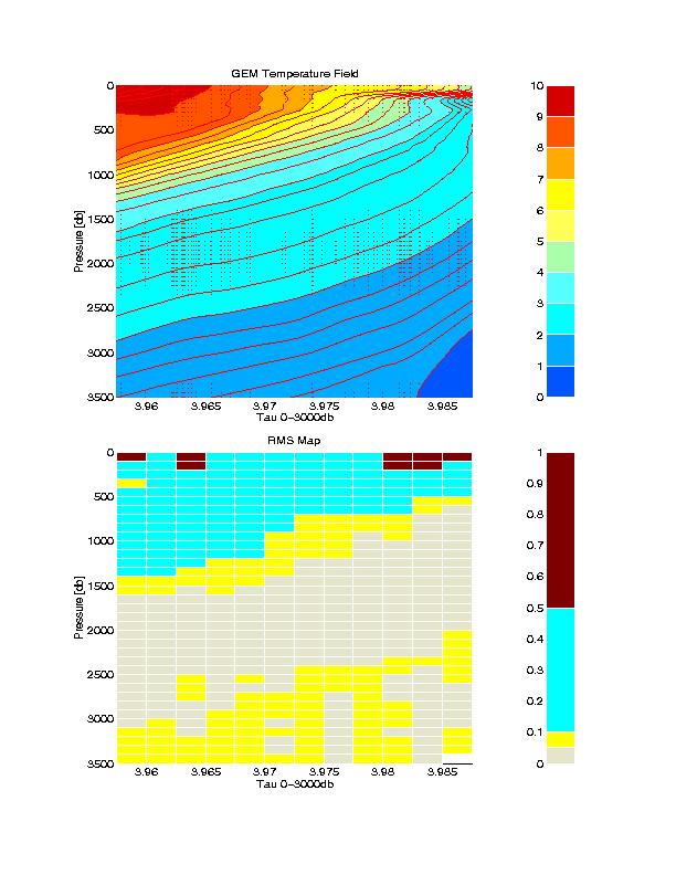
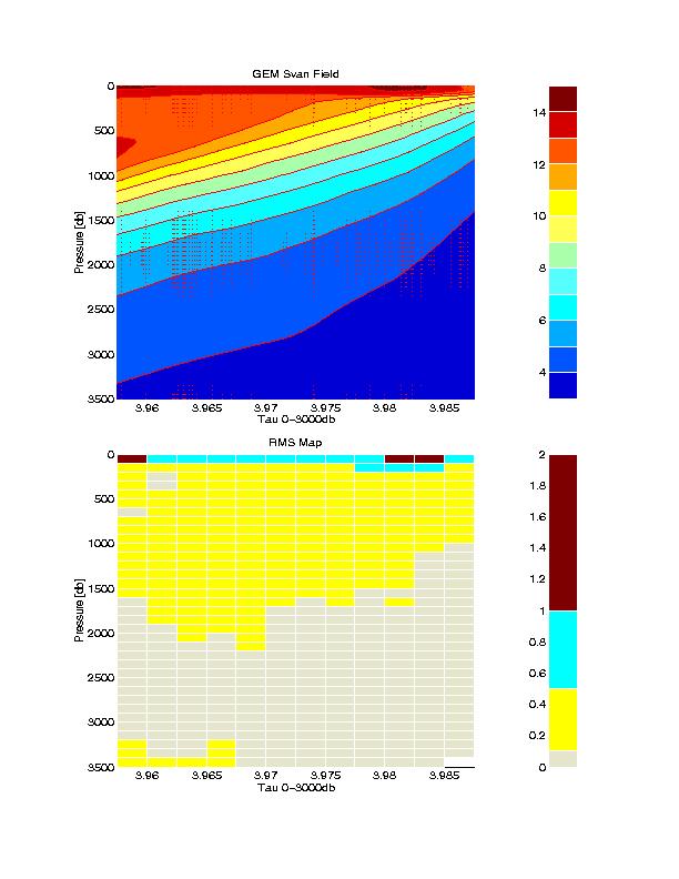
Hydrographic measurements, taken on 8 sections along the WOCE SR3 line and encompassing all four seasons, were integrated to obtain a value of tau for each cast. The corresponding temperature (T) profiles for all of these casts were then smoothed onto a regular grid of pressure and tau producing a smoothed field of temperature. Dotted lines indicate the individual casts. A smoothed field of specific volume anomaly (svan) was similarly produced. These fields show the dominant T and svan profiles associated with any given value of tau. The variation shown in these figures documents a single, dominant mode of variability which we refer to as the ``Gravest Empirical Mode'' or GEM. The word ``mode'' here does not refer to an analytical or dynamical mode, but to a purely empirical mode.
The lower panel associated with the temperature GEM field shows the root-mean-square difference (degrees C) between the actual CTD measured T values and the smoothed T field. The corresponding rms differences are also shown for the svan field. The highest errors are confined to the upper 200 dbars where seasonal fluctuations in temperature are large; however these have been reduced to less than 1 C by the seasonal model shown below. The scatter progressively decreases with depth and is uniformly small below the main thermocline. Within the 150-3000 dbar range, more than 97% and 96% of the T and svan variances, respectively, are captured by the GEM representation.
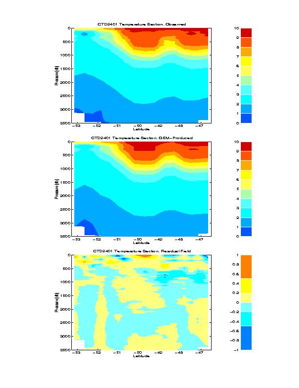
A GEM-produced temperature section across the SAF on the SR3 line captures the overall structure observed by CTDs. A CTD-measured temperature (in degrees C) section taken along the WOCE SR3 line during January 1994 is contoured in the upper panel. To produce the corresponding GEM-simulated temperature field in the middle panel, each CTD cast was integrated to simulate the tau measurement of an inverted echo sounder. The tau values were then used to calculate the corresponding T profile from the GEM smoothed field. The resulting T profiles are contoured using the same color scheme as in the upper panel. The difference between the two sections is shown in the bottom panel. Throughout the majority of the water column the differences are less than 0.2 C. By incorporating the seasonal correction into the GEM-produced temperatures the agreement in the surface layers is remarkably good.
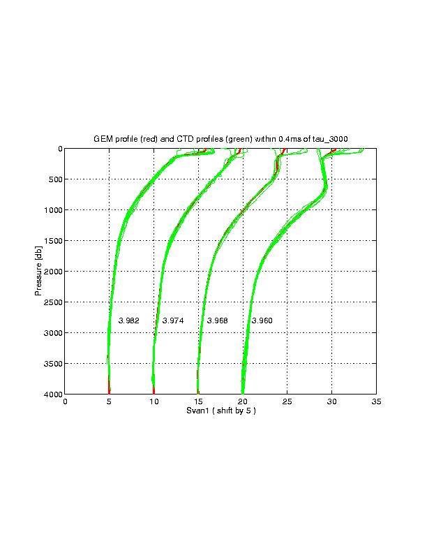
GEM-produced svan profiles at four representative tau values equal to 3.982, 3.974, 3.968, and 3.960 seconds are shown (from left to right) as bold red lines. The thin green lines are profiles of svan directly calculated from CTD data for casts within 0.4 milliseconds of the tau values. The largest differences occur in the upper 200 dbar where the seasonal temperature fluctuations are evident.
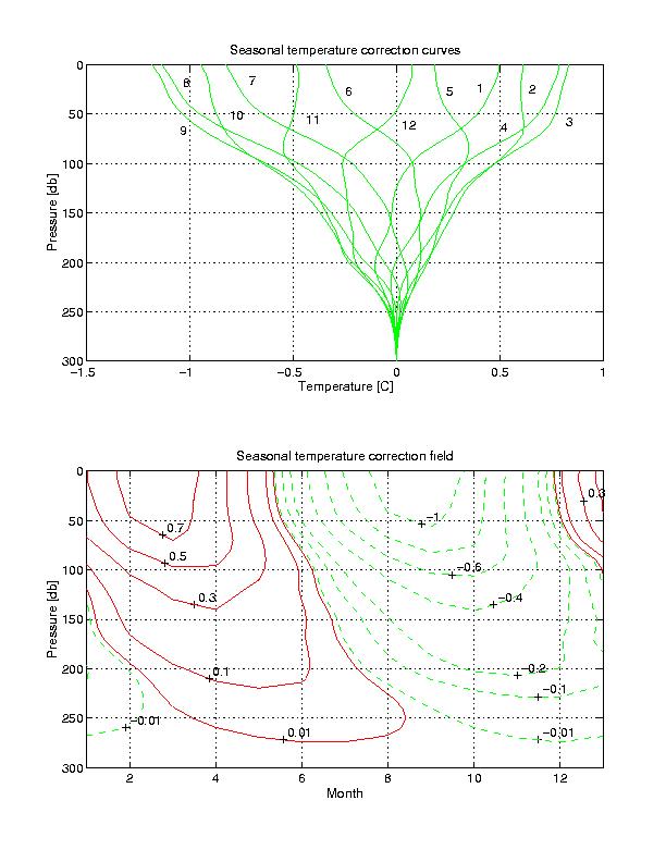
The GEM T and svan fields can be improved by taking into account seasonal changes in the surface layers. The average seasonal signal was determined using historical CTD casts taken along the WOCE SR3 line and casts taken in the surrounding region obtained from Alfred-Wegner-Institut fuer Polar-und Meeresforschung. The GEM profiles were removed from the measurements and the resulting difference profiles were grouped by month. The upper panel shows the monthly difference profiles for temperature within the upper 300 dbar (months are labeled by numerical values). The lower panel, which redisplays these same profiles contoured as a function of month, emphasizes the lag time required for the seasonal changes to propagate downward from the sea surface. Modifying GEM-derived profiles of T and svan by incorporating these seasonal changes greatly improves the near-surface agreement with measured CTD profiles, as shown in the rms difference plots.
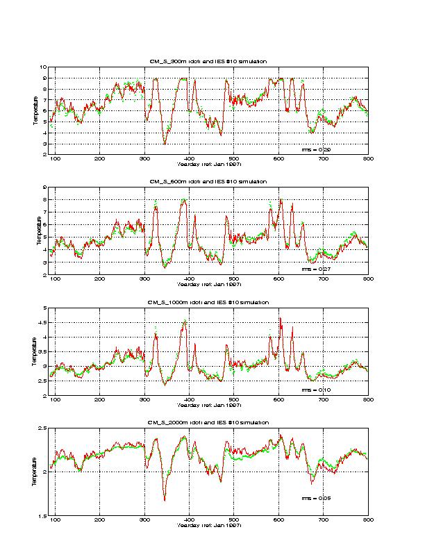
Three IESs sites coincided with current meter mooring locations. The 40-hour lowpass filtered travel time records from these instruments were used with the GEM methodology to produce temperature records at four depth levels at current meter mooring locations. The GEM-produced temperatures for the two-year-long (March 1995 to March 1997) time period at one location (CM_S) are shown by the solid red lines for the four depth levels. Temperatures measured by current meters are superimposed by the dotted green lines. The two methods agree within 0.3, 0.3, 0.1, and 0.05C at 300, 600, 1000 and 2000 m, respectively.
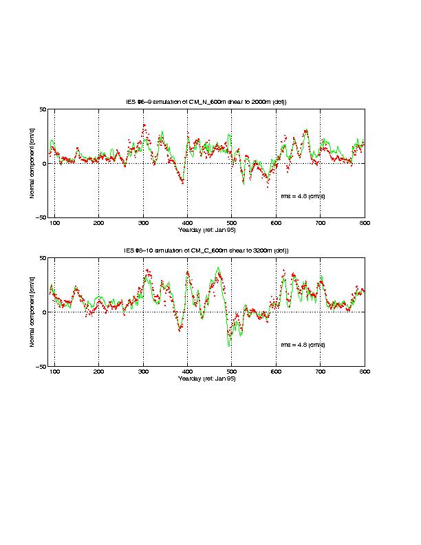
Measurements from two adjacent IESs can be used to determine the vertical profile of the component of horizontal velocity normal to the line between the two sites. Two-year-long velocity records were determined from the IESs for the sites of two current meter moorings, CM_N and CM_C, located along the western line of IESs. Independently observed shears were obtained by differencing the measured currents at 600 m and the deepest measurement depth on each mooring. The IES-derived velocities at 600 m relative to 3000 m (green solid lines) are superimposed on the directly measured velocity shears (red dotted lines). All velocities are the component along 108T, normal to the IES section. There is excellent agreement (rms of < 5 cm/s) between the two velocity estimates at both locations.
Two-dimensional arrays of IESs can resolve both components of velocity. Shown are the observed current shear vectors (lower panel) at mooring CM_C and the corresponding IES-derived velocity vectors (upper panel) for the March 1995-March 1997 time period. Cyan-colored upward-pointing vectors indicate northward flow and red vectors indicate southward flow. Note that the two types of measurements are not equivalent: the current meter velocities represent point measurements while the IES-produced velocities represent horizontal averages spanning the gaps between measurement sites. Additionally, since the mooring site is located along the western edge of the IES array, the component of velocity parallel to the line is not as well resolved as at locations near in the middle of the 2D array where both components of horizontal gradient are well determined. Nonetheless, the IES-derived velocities agree strikingly well with the directly measured currents in both speed and direction.
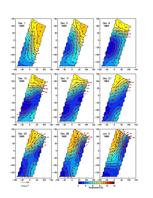
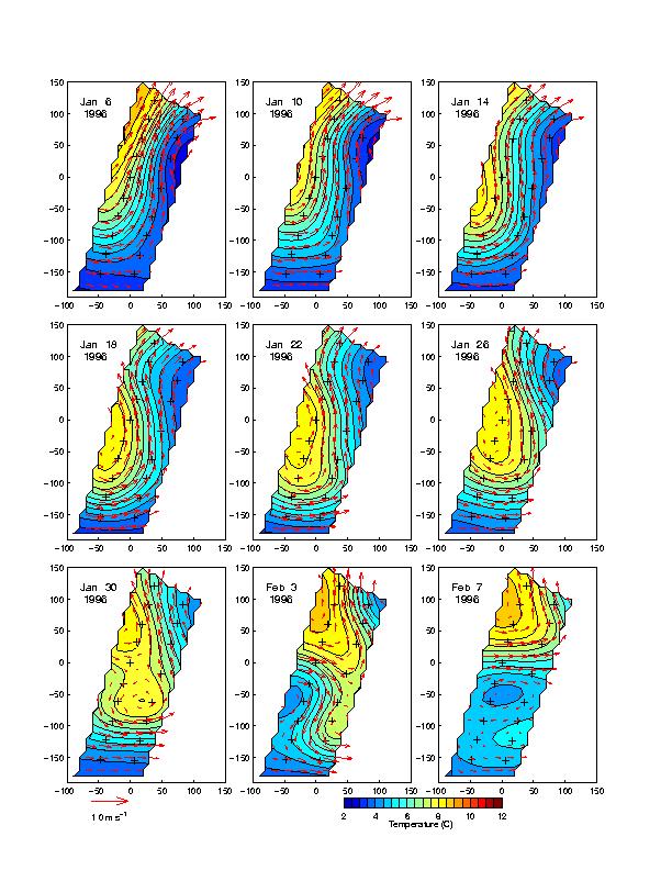
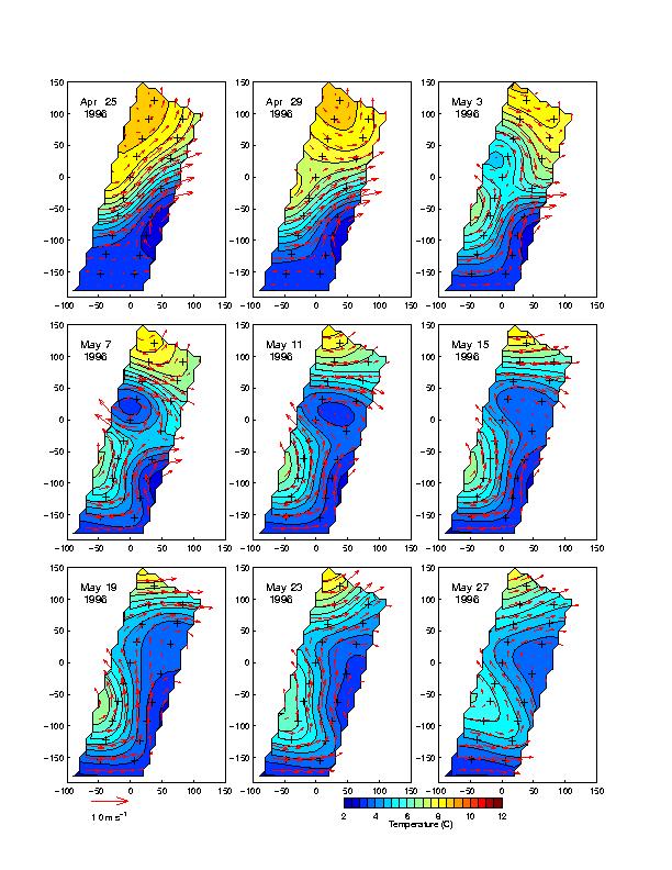
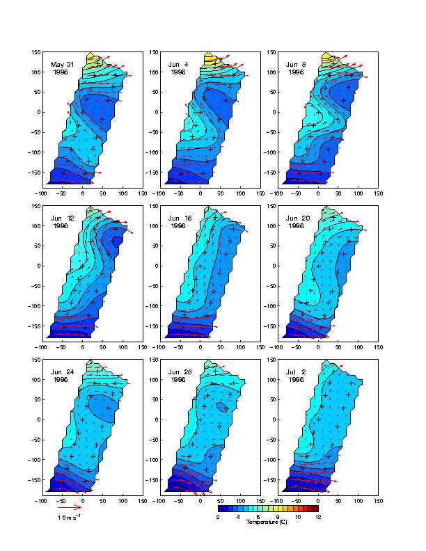
Optimally-interpolated maps of the temperature and velocity fields at 600 m depth measured by the IESs were produced at daily intervals for the full two-year time period. Two examples are presented which show the temperature fields at 4-day interval (color-coded according to the scale shown at the bottom of each figure). The IES sites are indicated by the plus symbols. The high velocities associated with the 7-9 C waters correspond to the Subantarctic Front and those associated with the colder 2-3 C waters correspond to the northern Polar Front.
This event illustrates a large meander trough of the SAF as it passes through the study region during a two-month period. On December 1, 1995 the leading edge of the meander trough is located in the mapping region and the flow of the SAF is oriented nearly north-south. During December 9--13 the primarily east-west flow in the upper portion of the array is associated with the passage of the base of the trough. From December 21 through January 10, 1996 the leading edge of a crest progresses through the array. During the latter part of January, this large meander crest may be forming a ring.
During this event the SAF and the northern Polar Front move apart. On April 25 the two current fronts are adjacent as a large meander passes through the array. During the month of May a cyclonic eddy moves eastward into the region, contorting the flow field and separating the two currents. During June the two currents are separated by 300 km---the flow associated with the SAF at the northern edge of the array while the colder Polar Front is at the southern edge.
For further information please contact D. Randolph Watts (rwatts@gso.uri.edu) by email. This poster was presented at the WOCE Conference in Halifax, Canada during 24-29 May 1998.
The GEM methodology has also been applied to measurements of the North Atlantic Current in the Newfoundland Basin. Connect to NAC transports for details of that application. A manuscript entitled "Vertical Structure and Transport on a Transect across the North Atlantic Current near 42 N: Timeseries and Mean" by C.S. Meinen and D.R. Watts, submitted in 1998 to the Journal of Geophysical Research, discusses the GEM and its application.
Go to URI's SAFDE page
Go to main SAFDE website
Go to the Dynamics of Ocean Currents and Fronts Homepage