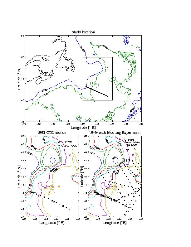
This first figure shows the location of the study
area . Left panel: Locations of the CTD profiles and POGO launches
from the 1993 CTD section aboard the R.V. Oceanus. Right panel:
Locations of the moored inverted echo sounders (IES) and deep current
meters deployed in August 1993 and recovered in April-June 1995. Also
shown in the right panel are the locations of other CTD profiles
obtained during the mooring experiment.
Three different methods of referencing geostrophic relative velocity
profiles were used after Pickart and Lindstrom [1994]: spatially
integrating the absolute velocity measurements of an Acoustic Doppler
Current Profiler (ADCP) horizontally between CTD stations; temporally
integrating ADCP measurements while on CTD sites; and using POGO
transport floats to provide the reference (the two ADCP methods were
modified somewhat from those used by Pickart and Lindstrom). The biases
between absolute velocity sections referenced by the different methods
were less than 1 cm/s and the standard deviations of the differences
were 5-7 cm/s.
For these three methods, the following sources of error were studied:
Ageostrophic velocities due to current path curvature, Schuler
oscillations in the ship gyrocompass, inertial oscillations, ADCP
misalignment error, GPS accuracy (including dithering), Ekman
velocities, scatter in the ADCP measurement, ADCP amplitude coefficient
error, heading dependent gyrocompass error, spatial sampling errors,
and POGO velocity measurement error. Based on estimates of the sizes of
all of these sources of error during the experiment, we determined that
the use of the POGO transport float to provide absolute referencing for
geostrophic relative velocity profiles resulted in the smallest
estimated error at all three CTD-pair spacings tested: 20 km, 40 km,
and 60 km. During the 1993 cruise, referencing via the POGO method
resulted in absolute velocities accurate to within 4 cm/s.
The next figure shows the resulting velocity
sections . Panel A shows the absolute velocity section for the 1993
section using the best available method for each CTD pair (the POGO
float failed for two CTD pairings). The green shading and dashed
contours indicate southward velocities, the medium blue denotes
northward velocities less than 50 cm/s, and the light blue denotes
northward velocities greater than 50 cm/s. Contour level is 10 cm/s.
Red circles on lower axis indicate CTD sites. Gray shading indicates
the ocean bottom. Panel B shows the vertical average of the absolutely
referenced horizontal velocity. The error bars indicate the accuracy of
the absolute reference velocity. Green shading indicates southward
velocity, blue indicates northward.
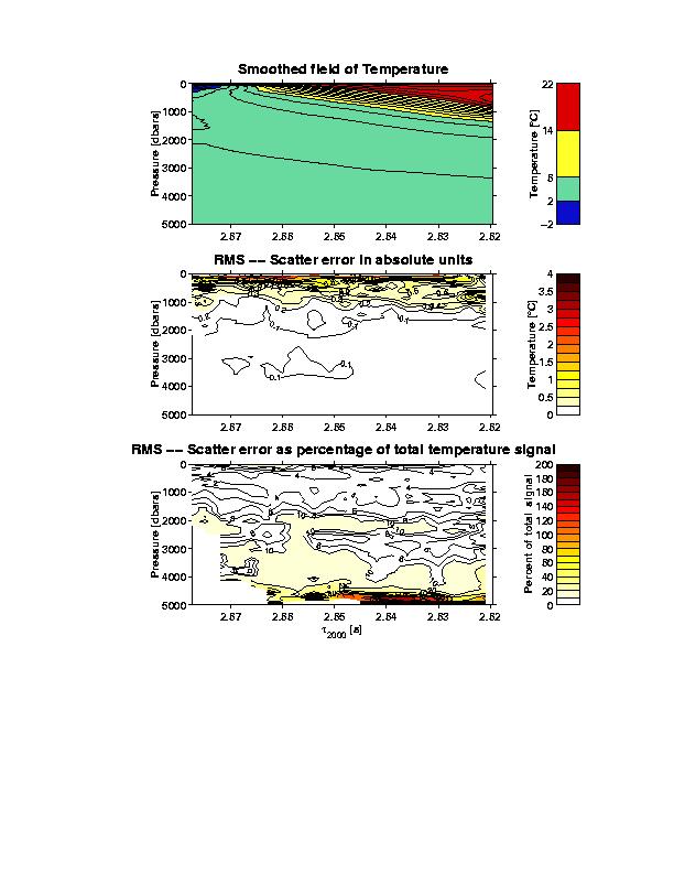
Hydrographic measurements from the Newfoundland Basin (shown on the
site map) were integrated to obtain a value of tau (round trip travel
time) for each cast. The corresponding temperature (T) profiles for all
of these casts were then smoothed onto a regular grid of pressure and
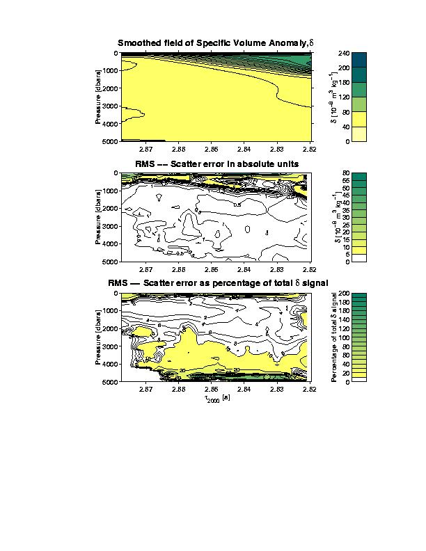
tau. A smoothed field of specific volume anomaly (delta) was similarly
produced. These fields show the dominant T and delta profiles associated with any given value of
tau. The variation shown in these figures documents a single, dominant
mode of variability which we refer to as the "Gravest Empirical
Mode" or GEM. The word "mode" here does not refer to an
analytical or dynamical mode, but a purely empirical mode.
The scatter about these smoothed temperature and delta fields is
quantified in the subsequent plots. The middle panels show the
root-mean-square difference between the actual CTD measured T values
and the smoothed T field in absolute units. The highest errors are
confined to the upper 300 dbars where seasonal fluctuations in
temperature are large. The scatter progressively decreases with depth
and is uniformly small below the main thermocline.
The total range of T and delta values vary with pressure level, with
the largest range in the main thermocline levels and smallest in the
deeper waters. Thus the bottom panel shows the same rms differences but
normalized by the total (peak--to--peak) T range at each pressure
level. The scatter in the thermocline region represents less than 5% of
the total signal for both temperature and delta; only in the deepest
waters where the actual temperature signal becomes very small does the
scatter exceed 10%.
Six sample plots detailing the temperature
(shading) and velocity (contours) structures observed on the dates
shown. Velocity contours are at 10 cm/s intervals, with bold contours
at intervals of 50 cm/s. The weak currents shown in the left panels,
with peak velocities of only 60 cm/s, result from oblique crossings of
the moored section by the North Atlantic Current. The methods used here
only determine the normal component of the velocity. The upper right
panel shows a more normal velocity section, with peak speeds of over
100 cm/s. The middle and lower panels on the right show the extremes of
the effect of the Mann Eddy on the apparent velocity of the North
Atlantic Current. In the middle panel the eddy is nearly separate from
the North Atlantic Current while in the bottom panel the two northward
flows are completely coalesced, with peak velocities of over 160 cm/s.
The North Atlantic Current and the northward flow of the Mann Eddy are
generally indistinguishable, like the right top and bottom panels. On
brief occasions the eddy moved shoreward enough that the southward flow
of its eastern edge was observed by our moored instruments, as in the
bottom right panel.
Based on these daily pictures the stream-coordinates
mean temperature and velocity sections were determined. Velocity
contours are at 10 cm/s intervals, with bold contours at intervals of
50 cm/s. Temperatures are displayed in degrees C. The
stream--coordinates origin was defined as the 10 C isotherm at 450
dbars. Nineteen months of daily measurements were averaged; time
periods when the North Atlantic Current was crossing the moored section
obliquely by more than 20 degrees, approximately 30% of the time
series, were excluded prior to averaging.
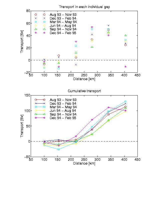
The next figure shows the absolute transport
across the section in different seasons as calculated from the
moored instruments. The top panel shows the net transport (northward
minus southward) integrated in each gap between moorings individually.
The bottom panel shows the cumulative integrated transport (northward
component only!), with the integration beginning at the second mooring
from shore. The inshoremost mooring was neglected in order to focus on
the northward transport associated with the combined North Atlantic
Current and Mann Eddy.
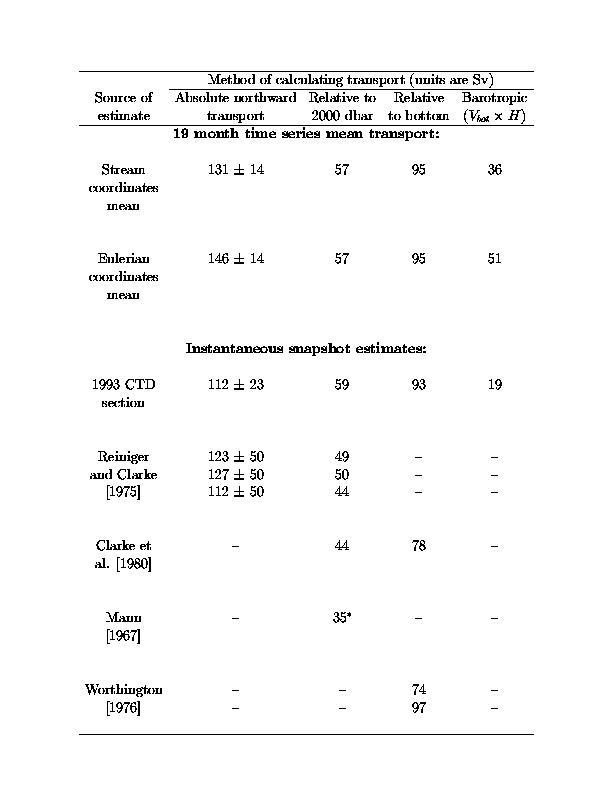
Different estimates of the NAC transport are listed in this table. Asterisk -- Mann's estimate does
not include the transport of the so-called ``Mann Eddy'' as it had
moved away from the NAC during his study. Reiniger and Clarke [1975]
used 24 hour averages from moored current meters to reference three
separate geostrophic shear sections from hydrographic sections. Clarke
et al. [1980], Mann [1967], and Worthington [1976] worked solely with
unreferenced geostrophic shear sections based on hydrographic
measurements (Worthington had two sections).
The absolutely referenced estimates of the transport agree to within
the accuracy of the various estimates. Because most of the historical
transport estimates were made relative to the assumption of a level of
no motion at 2000 dbars or at the bottom, these transport values are
shown also. There is fairly good agreement between these various
estimates as well. Note the importance of the bottom velocity component
of the transport however. It represents 17-35% of the total transport!
The reduction in transport when calculated in stream--coordinates was
unexpected. Work with a simple analytical model of an eddy indicates
that, since the Mann Eddy does move with respect to the core of the
North Atlantic Current, the stream--coordinates averaging would result
in the averaging of some of the northward flow of the Mann Eddy with
some of the southward flow of the eddy. The result would be a lower
northward transport, as was observed. For this reason the Eulerian
transport estimate was used for comparison to other transport estimates
in the northwest North Atlantic.
The combined northward absolute transport of the North Atlantic Current
& Mann Eddy was observed to be about 145 Sv at 42.5N. This is
significantly larger than historical (non--absolute) estimates at this
location, which prompted us to reconsider the overall circulation ideas
for the northwestern North Atlantic. This
sketch indicates a possible circulation scheme for this region. The
numbers indicate transport estimates in Sverdrups (1 Sv = 1000000
m^3/s) made in this and other studies. All of the transports are
absolute except for the estimate of the eastward transport across the
Mid-Atlantic Ridge, where no absolute estimate has ever been made.
Several studies have suggested, however, that the level of no motion
assumption at the bottom may be valid crossing the Mid-Atlantic Ridge,
so this estimate is treated as robust.
Historical estimates of the recirculation within the Mann Eddy give
50-60 Sv; hence the difference, 90 Sv, is identified as the throughput
northward transport of the North Atlantic Current on this transect.
With 90 Sv entering this part of the North Atlantic Basin and only 30
Sv leaving over the ridge, significant southward recirculation must
occur elsewhere in the Newfoundland Basin in addition to the
recirculating Mann Eddy. Potential pathways for this recirculation are
shown by dashed lines. A number of float studies have shown no evidence
for southward recirculation offshore of the North Atlantic Current.
This is a region of high eddy variability, however, and the mean
velocities needed to produce our hypothesized southward recirculation
are so small (0.5 cm/s) that it is unlikely that they would be easily
observed.
For further information please contact Christopher Meinen (meinen@pmel.noaa.gov) or D. Randolph Watts (rwatts@gso.uri.edu) via email. This poster was presented at the WOCE Conference in Halifax, Canada during 24-29 May 1998.
The GEM methodology has also been applied to measurements in the Subantarctic Front south of Tasmania. This highly successful application was the subject of another poster at the WOCE conference.