The ARIANE Lagrangian diagnostic more in detail
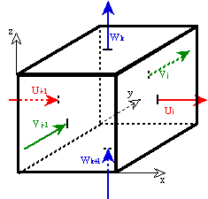
The analytical calculation on a C-grid of three-dimensional streamlines, for periods over which the velocity field is assumed to be constant, defines a convenient way to derive particle trajectories within any model gridcell.
The equations
• Three basic relationships are written (here for x):
![]()
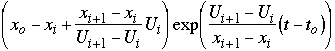
• Integrating this equation gives:
![]()
• The crossing time in the zonal direction is:
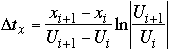
• The final position on the edge of the gridcell is defined from the minimum of Ætx, Æty, Ætz.
The best positioning of the particles over initial sections is the one that gives the highest accuracy of the transports we compute, for a reasonable number of initial positions (see Blanke and Raynaud, 1997). We can evaluate the accuracy as the difference between "section to section" transports obtained for a forward then a backward integration, as both transports are virtually equal.
Following a set of particles in the ocean and summing their algebraic transport at each velocity gridpoint, we obtain a 3D field that corresponds to the flow of the water mass in study (Blanke et al., 1999). As one particle entering a model gridcell by one of its six faces has to leave it by another face, the transport field satisfies
¶iTx + ¶jTy + ¶kTz = 0,
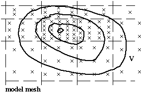
where Tx, Ty and Tz designate the directional flows in sverdrups. Integrating this field along a selected direction, we obtain a 2D non-divergent field that we study by means of a streamfunction.
Therefore, ARIANE lead to:
Individual trajectory computations
- extensive use of the output of an Ocean General Circulation Model (OGCM);
- finite differencing on a C-grid expresses mass conservation in a very natural way: it states that entering mass in a given gridcell must be balanced by an exactly equal outflow;
- ideal framework for the computation of analytical mass-preserving streamlines (Blanke and Raynaud, 1997), for a given sampled velocity field;
- successive segments of such streamlines are associated to actual three-dimensional trajectories of fictive fluid particles, assuming the velocity constant over periods equal to the sampling time of the output.
Quantitative transport estimates:
- obtained by increasing the number of particles, following the methodology introduced by Döös (1995);
- due to water incompressibility, one given particle with an infinitesimal volume is to conserve its infinitesimal mass along its trajectory;
- the transport of a given water mass is calculated from its own particles and their associated infinitesimal transport;
- the best initial positioning is obtained by grouping particles in regions where the transport is the highest.
Pathways visualisation (Blanke et al., 1999):
- calculation of the three-dimensional non-divergent transport field determined by the displacement of the particles and their associated transport;
- projection on a given (horizontal, zonal, or meridional) plane;
- diagnostic and plot of the associated streamfunction.
A few words about accuracy and methodology:
- off-line diagnostics allow backward computations of trajectories (simply by multiplying all velocity outputs by -1, and reversing their chronological order);
- the joint use of backward and forward calculations provides a measurement of the error made on computed transports, as they define independent estimates;
- off-line Lagrangian diagnostics permit to loop over a climatological year when calculating trajectories, without the constraint of the true length of the OGCM simulation for setting up the limits of the Lagrangian integration.
|
|
|
|
|
|
|
|